We’re hoping that this series on linear regression will help if:

• You’re looking to get started in analytics and/or move across from an adjacent field
• You’re in a position where you need to interact with an analytics team
  and want to increase your vocabulary and communicate better
• You’ve heard the term “machine learning” and need to start from the beginning
• You want to understand the basis of predictive or forecasting techniques.

Whichever is the case we’ll be explaining the techniques, what they do, how to use them and how to analyse their outputs. We’ll also give code examples in R (We’ll cover R in more detail in a future post).

We will try to explain what’s happening with words and pictures as far as it’s practical, however, a bit of maths is unavoidable.

We are going to assume around about high school level maths, basic calculus, linear algebra and probability, but otherwise try to build things up from first principles.

What is Linear Regression and why is it important?

Regression covers a broad range of techniques where we estimate to what extent a variable of interest, often called the dependent or responding variable, can be predicted by a number of known variables, often called the manipulated or independent variables. While there are many regression techniques available to the Analyst, covering a variety of different situations, they are all extensions of the simple linear regression technique covered here.

Example – Test Scores

Let’s start with a simple (and almost canonical) example. We have the test scores of 40 students.

Table 1: Test Scores

63.7	71.8	61.6	86	73.3	61.8	74.9	77.4	75.8	66.9
85.1	73.9	63.8	47.9	81.2	69.6	69.8	79.4	78.2	75.9
79.2	77.8	70.7	50.1	76.2	69.4	68.4	55.3	65.2	74.2
83.6	69	73.9	69.5	56.2	65.9	66.1	69.4	81	77.6

A typical use of simple linear regression centres around the question: “How do I grade a student that has missed this test due to absence, what score should they be assigned?”.

If the only information we have are the other students’ test scores then the best we can do is give the student the average or mean score:

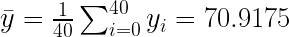
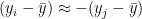
There is a valid criticism to this approach: If the sick student was a star student then shouldn’t they receive an above average mark for the test? Likewise, should a normally below average student receive the average?

What if, in addition to the latest test scores above, we had scores for each student’s previous test?

Table 2: Scores for the two tests as ordered pairs (old score, new score)

(17.2, 63.7)	(19.8, 71.8)	(18.2, 61.6)	(26.2, 86)	(19.4, 73.3)
(15.5, 61.8)	(22.1, 74.9)	(23.7, 77.4)	(21.4, 75.8)	(20.4, 66.9)
(25.6, 85.1)	(19.8, 73.9)	(18.3, 63.8)	(10, 47.9)	(26.3, 81.2)
(23.5, 69.6)	(18.9, 69.8)	(20.8, 79.4)	(23.6, 78.2)	(21.4, 75.9)
(27.6, 79.2)	(22.3, 77.8)	(21.3, 70.7)	(13, 50.1)	(20.3, 76.2)
(19.9, 69.4)	(15.5, 68.4)	(17.6, 55.3)	(18.4, 65.2)	(25.5, 74.2)
(25.2, 83.6)	(17.9, 69)	(22.2, 73.9)	(17.7, 69.5)	(12.5, 56.2)
(18.9, 65.9)	(17.5, 66.1)	(19.5, 69.4)	(23.6, 81)	(21.1, 77.6)

If we look at figure 1, illustrating the old and new test scores of the original 40 students, then we can see there is clearly a relationship between students’ scores on the two tests (students who did well on the last test tend to perform well on the next test).

Figure 1 – Old and new scores for each student

If the sick student scored 25 on the old test then a score of 80 seems reasonable (gold line), likewise a score of 15 on the fist test might correspond to a approximately 60 on the new test.

Intuitively, if we want to assign a score to a student who has missed a test we could ’eye ball’ this chart. If the student scored 15 on the first test then a guess of 60 for the second test seems reasonable (blue lines on our plot), similarly the if the student scored 25 on the first test then assigning a score of 80 on the second test seems reasonable. This brings us to the crux of regression, what we want to do is take this idea of “eye balling” the chart and add rigour and precision.

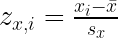
Z-scores

If we look at our data, so far we see that our two tests have a different ranges, the later test scores vary from a little below 50 to just over 85, while the earlier test scores vary from around 10 to 28. Continuing with calling our new test scores and labelling our older scores we calculate our means, (as above) and .

Next we calculate the standard deviation.

We have for the old tests and for the new . In later post we’ll dig a little more into standard deviations and the insight they provide about how our data is distributed (under certain conditions), for now we’ll take this as a measure of how spread out out our data is. Next we calculate scores for each of our test scores (old and new with defined analogously):

The score tells us how far a score is from the average score, in a way that doesn’t depend on average or spread of scores (it is simple to show that the average of the scores is always 0 and the standard deviation is always 1).

The advantage of this is that we can now compare scores from the old and new tests on the same footing. Lets plot our scores for the two tests, in fig 2 we see that the two sets of scores now have a similar range and our problem has been simplified to this: for a student that has scored above or below average how far above or below average should do we expect them to perform on the next test . We could do this by having a linear relationship between the two scores that was a good ”representative” of the data – unfortunately the blue and gold lines both seem like they could be the ”best” fit.

To make this precise we will define the ”best line” as the one that minimises the square of the distances between the points and our line (see fig. 3)

Finding our line

We want to find the line (where will be our estimate for ) that minimises the square distance between and .

Figure 2 – Z scores with “best” fit lines estimated by eye

Figure 3 – Z scores with errors (dotted blue lines), the “best” line will be the one where the sum of the squared distances is minimised

We have:

To minimise we want both our derivatives: and to be zero.

Where we have made use of the fact that 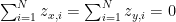. The derivative with respect to :

We now look at the numerator and the denominator separately.

gives you.

(where the covariance )this value has a special name we call it the “Pearson correlation coefficient“, it is usually denoted or (and sometimes called Pearson’s r or simply the correlation coefficient). To understand what it tells us and why it is useful lets transform back to and (our test scores from earlier). 

We have: 

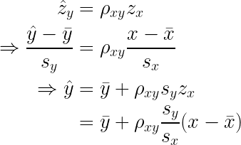
What does this mean?

This equation gives us a procedure for estimating for a given value: first calculate the z score of multiply the result by and add the result to the mean value of .

In order to really understand this lets look look at two extreme cases:

In the first lets assume that , for this to happen for each pair there is a nearby pair such that and . In our testing example this means that for every student performing well on both tests there is a student performing equally well on the first test then poorly on the second e.g the first test tells us little about the second. In this case and our estimate for the second test will be the average score (i.e. the bets guess we could make when we didn’t have the older test scores). 

In the second extreme case imagine that the second test could be perfectly calculated from the first with a linear relationship, for some and . In this case:

Where is 1 if is positive, -1 is is negative and 0 if is zero. In this case our procedure for estimating a new value is (unsurprisingly):

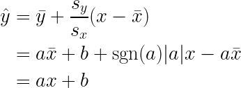
i.e. For a new score we work out how many standard deviations it is from and estimate as being the same number of standard deviations from .

In reality sit somewhere between these two extremes, with values close to 1 indicating a strong positive relationship, values close to -1 indicating a strong negative relationship and values close to 0 indicating no relationship. If is close tells us that our estimate should be based primarily on a linear relationship between the variables, values close to 0 tell us that there is a weak relationship between the variables and we should simply take the mean of our dependent variable (ignoring the unrelated independent variable). For values in between gives a balance of the two approaches, or how far we should regress back towards using a mean value for our estimate.

So … what score does the student get?

For the set of values above we get which indicates that there is a strong (but not perfect) positive relationship. If our sick student hypothetically score 15 on the old test then following our estimation procedure gives us , similarly an old test score of 25 gives and estimate (both of which are pretty close to our “eye ball” estimates).

So now we have a method for deciding whether there is strong linear relationship between two variables, and a procedure for estimating a responding variable (like our test score) based on an independent variable (our old test scores).

What we haven’t talked about yet is errors, which we’ll leave for another post. In particular to really understand regression and hence know when you can and can’t use this technique we’ll need to cover:

• What do we mean by “best fit”?
• Why did we take the square distance between our scores and our estimated line? Is this always the “best” fit?
• How can we calculate the uncertainty in our predictions?
• How small does get before we can say there is no relationship?

Once we have covered these we’ll have our first tool under our belt. Finally it’s worth noting that simple linear regression has a number of real world applications and we’ll talk about some of these in future posts.